Modelling RPI & CPI Volatility in Financial Canvas

Having recently joined the Financial Canvas team, I expected the process of extending the CPI and RPI model to be extremely challenging. However, using the Financial Canvas model building system and software, it was surprisingly intuitive and enjoyable!

The new approach to modelling RPI and CPI gives them both some shared, correlated volatility and then, to each of them, orthogonal volatilities derived from past correlation.  

This better captures the realised inflation series, including some CPI "basis risk" for pension increases linked to CPI with investments using index linked gilt assets linked to RPI.

I carried out the process in two stages.  Firstly, a workflow using existing blocks to carry out statistical operations in sequence, and then creating a single block responsible for to replicating the entire workflow:

Prototyping Implementation vs New Streamlined Block

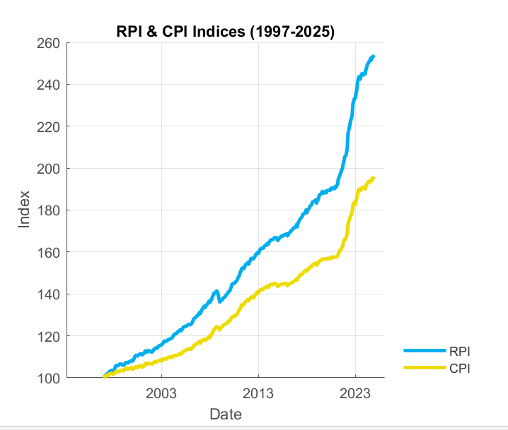
Exploring the Historical Data

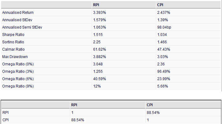
First, I downloaded the historical RPI and CPI series from the Office of National Statistics to pull through Financial Canvas and gain some insight into their historical features. I found for the period 1997-present:

-   Annualised volatility of RPI: 1.6%

-   Annualised volatility of CPI: 1.4%

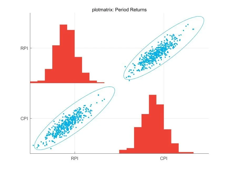
-   Correlation of RPI/CPI: 89%

These reference values formed the benchmark for our model.

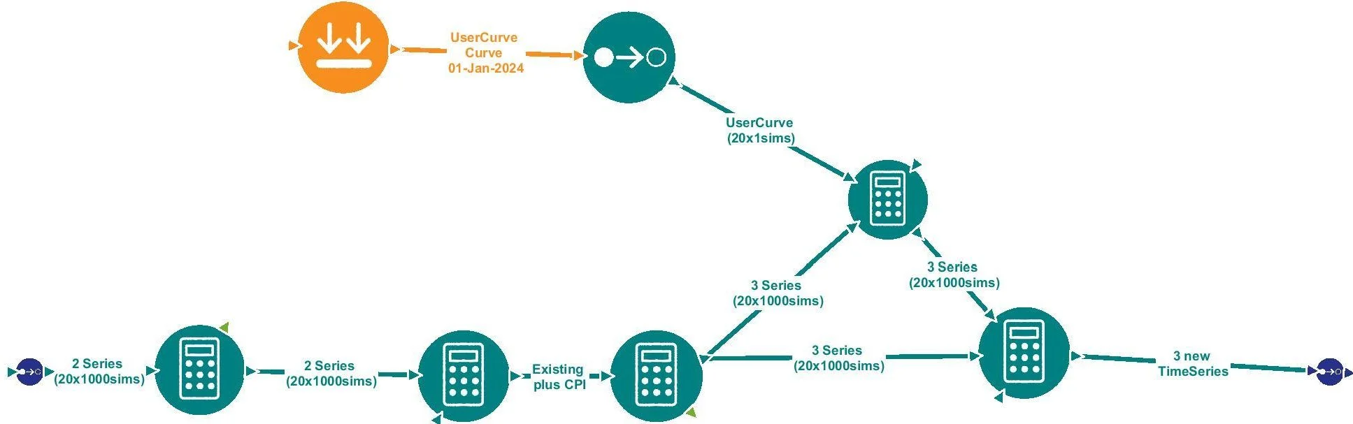
Building the Workflow

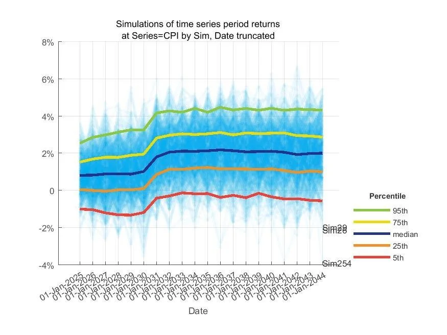
I then loaded an existing calibration model and forked the process after a preliminary RPI series had been generated from a series of inflation curves. This preliminary series derives realised RPI for each period from the front of the preceding breakeven curve.  This captures "anticipated" RPI volatility for each period of around 1.1% per annum; we then want to add the "surprise element" bringing the RPI volatility up to the historic target.

Using a series of 7 blocks, I developed a workflow and analysis to first add some ‘shared’ volatility, then split CPI from the first series and knock off the pre-RPI-harmonisation gap, and finally added some ‘orthogonal’ volatility to reach the target values.  The drag-and-drop nature of the model and easy developer access to the underlying methods made this easy to explore different ideas before settling on the final approach.

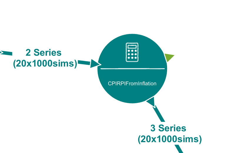
I set about on compacting this process into a single, new block, specifically in charge of creating desired CPI and RPI series. Using existing methods in the Financial Canvas toolbox and creating some of my own, I cut the workflow down from the 7 blocks to 1, handling just 4 simple steps:

1. Add a first volatility addition to Initial Volatility in order to reach a Shared Volatility compatible with the target correlation

2. Make a copy of the RPI series, renaming it CPI.

3. Knock off the RPI-CPI gap (0.9% of annual returns until 2030) from the new CPI series.

4. Add their respective "Orthogonal" Volatilities, to reach target CPI/ RPI volatilities.

Inputs and Outputs

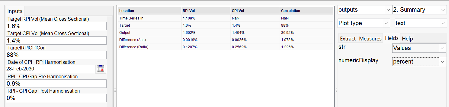
The block takes as input:

-   An RPI series derived from a series of inflation curves

-   Metrics

    -   Target RPI Volatility

    -   Target CPI Volatility

    -   Target RPI/CPI Correlation

-   Harmonisation description

    -   Pre-Harmonisation RPI-CPI Gap

    -   Post-Harmonisation RPI-CPI Gap

    -   Harmonisation dates

And outputs an RPI and a CPI series with target metrics and harmonisation.

Financial Canvas' clean and logical design philosophy gave me the freedom to experiment rapidly, while supporting the robust implementation of complex stochastic logic. It felt extremely satisfying to apply the maths and statistics from my degree to the real world 🤓

Look out for my future work where I will be integrating this approach into our core asset model and identifying further opportunities to validate and refine our stochastic asset models...